The covariance of two variables a and b is defined as
where we use 〈…〉 to indicate averaging. So, e.g. the average of a is 〈a〉 and so forth. By expanding the brackets and taking the average of each summand this can be simplified:
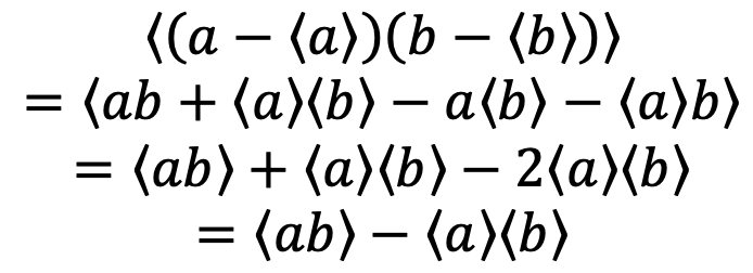
Using the definition of the fluctuations as deviations from the mean
We can write this as
From the the right hand side of this equation we see that
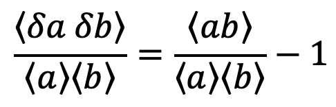
The left hand side is called the correlation coefficient of the fluctuations of the signals of a and b. The first term on the right hand side is the correlation coefficient of the signals a and b. As can be seen the two differ only by an offset of a value of one and are otherwise identical.
If the two variables are independent, then they are uncorrelated and the covariance is 0. Therefore,
If the two variables are correlated then the covariance is > 0,
If the two variables are anti-correlated then the covariance is < 0,
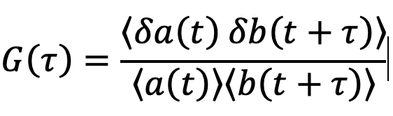
In general, the signals are recorded as a function of space, time, etc. Taking time t as an example we can write the correlation coefficient with the dependence on time indicated:
This provides us now the possibility to compare not only fluctuations that were measured simultaneously, giving us one single correlation coefficient, but we can now write this as a correlation function comparing fluctuations at different but fixed distances in time τ, the so-called lag time. At each value of τ the correlation function G(τ) tells us how the fluctuations δb(t+τ) depend on the fluctuations δa(t) a time τ earlier:
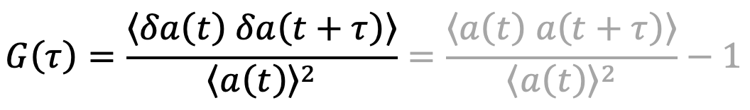
If we are interested on how fluctuations depend on past fluctuations of the same signal, we can define the autocorrelation function:
We need now one last piece to get to our final result. As we discussed under "Fluctuations", one of the advantages of FCS is that it can measure in equilibrium, i.e. at a staionary sample. Stationarity means that the average of the signal does not change with the time it is measure, meaning
The autcorrelation function (ACF) can thus be written as

In the graph above you see the principle behind the autocorrelation function (ACF). We compare the signal (blue) against its own copy (yellow) shifted in time by a lagtime τ. At small τ, there is considerable overlap for the whole signal and thus a strong correlation. With increasing τ this overlap reduces and the correlation function decreases until any overlap is due to pure coincidence (i.e. single peaks at different positions in the signal overlap but not all peaks overlap at the same time anymore).
Note that the lagtime τ can be positive or negative and the ACF is symmetric. To see that, replace τ with -τ in the ACF:
As we measure in a system in equilibrium or at least in a stationary state (i.e. mean and variance do not change in time) we can shift the time at which we measure the correlation function from t to t+τ. Substitution in the equation above shows that the ACF is symmetric in time: